We consider one‑step ahead forecasts with our first estimation window from Q1 1959 to Q2 2003. We commence with a brief review of the literature on consumption forecasting in section 4.1. We then outline the data in section 4.2 and follow this with the methodology in section 4.3. The section closes with the forecast and bootstrap prediction interval results.
4.1 Benchmarks
To develop suitable benchmarks, we briefly review the main models used for consumption forecasting and the variables employed. Given consumption is I(1), Autoregressive distributed lag (ARDL) models typically model the consumption growth rate as a function of lagged covariates (also in growth rates or first differences if I(1)). Depending on the lag structure, multi-step forecasts may be performed directly or iteratively, with the latter requiring externally generated forecasts of predictors. ARDLs perform well when the relation between variables is uncertain (Marcellino and Schumacher 2010) and whilst they can handle I(1) variables, the precondition that regressors are not I(2) or higher is often breached (Haldrup 1998). Factor models are also popular as they allow a large amount of information to be incorporated parsimoniously, however this comes at the cost of interpretability (Stock and Watson 2002; Andreou et al. 2013). Finally, Vector Autoregressive (VAR) and Vector Error Correction Models (VECM) are also common, with the latter explicitly allowing for cointegration which may improve longer term forecasts (Barlas et al. 2021).
Most papers employ variables like wage growth, wealth, interest rates and inflation. Alternative indicators like consumer sentiment and financial market data are also becoming more common. Whilst the effect of consumer sentiment is consistently significant, it is often modest in size (Carroll et al. 1994; Ludvigson 2004).1 Financial market data is of interest given its forward-looking nature, with the mixed results possibly due to conversion of the data to a lower frequency (Andreou et al. 2013; Stock and Watson 2003; Harvey 1989; Grasso and Natoli 2018).
More recently MIDAS models with high-frequency consumer sentiment and financial market variables have been shown to improve forecasts (Gil et al. 2018; Vosen and Schmidt 2011). Other promising high-frequency variables include Google Search trends and transaction level data (Barlas et al. 2021; Choi and Varian 2012; Duarte et al. 2017). To use the information available in large data sets, MIDAS typically employs dynamic factors (Bok et al. 2018) and model combinations (Gil et al. 2018), with equal weights often outperforming more sophisticated strategies (Soybilgen and Yazgan 2018).
4.2 Data
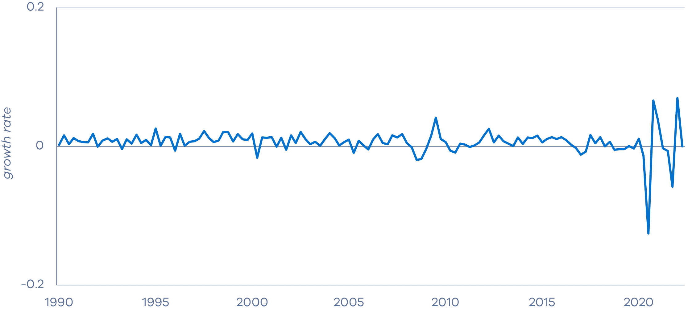
Table 1 provides details on the data and its sources. We employ the latest vintage as consumption is revised on average less than half a percentage point from the original release, and data vintage has little effect on forecast performance (Bishop et al. 2013). Where required we collect seasonally adjusted variables and deflate nominal variables using the implicit price deflator published by the ABS. For financial market data, the small number of data gaps employ a past-value backfill. Excluding the VECM models, all I(1) series as identified by Augmented Dicky-Fuller tests are logged and first differenced. Refer to Table 5 in the Appendix for a complete list of transformations and summary statistics.
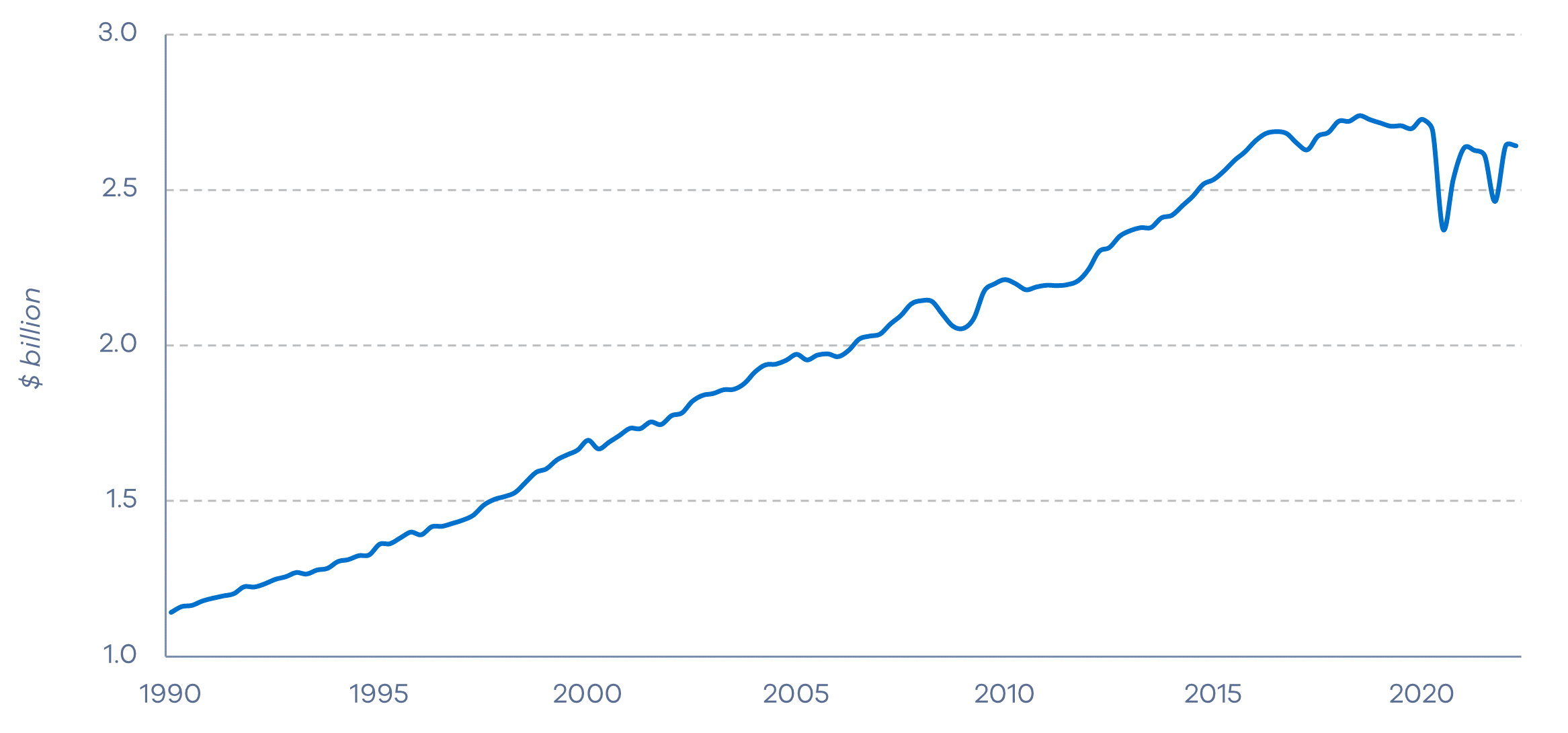
Figure 1 plots quarterly real seasonally adjusted final household consumption. The series has grown considerably since 1990 with falls during the Global Financial Crisis (GFC) and COVID-19 pandemic. The GFC is considered to start Q1 2008 and end Q2 2009. Although there is consensus on the GFC end date, the start date is unclear (Do et al. 2018), so our start date is based on structural break tests. Structural break tests also indicate the COVID‑19 pandemic starts Q2 2020 and continues until the end of the series.
The dataset contains variables measured at the quarterly, monthly, and daily frequency. The majority of regressors are monthly, and wage growth, consumer sentiment, job ads and house prices2 are an index. Starting points differ, with most series available from 1990 onwards. For model estimation, the widest window of available data has been used.
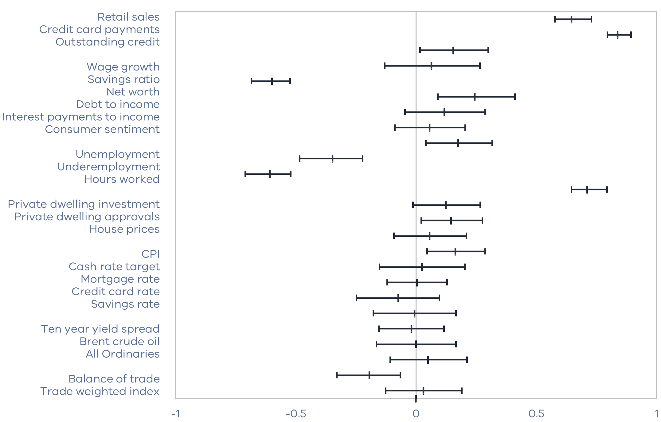
Figure 2 presents the correlation of each variable with the growth rate in consumption. A number of spending activity measures are highly correlated with consumption, in particular retail sales (0.65) and credit card payments (0.84). Inflation, interest rates and household finance variables have low correlation. For example, consumer sentiment (0.18), the CPI (0.16), and many financial market indicators have low correlations and 95 per cent confidence intervals that span zero.
Table 1: Summary statistics
| Frequency | Series start | Units | Mean | St. dev | Source | |
|---|---|---|---|---|---|---|
| Consumption | Quarterly | 1959 | $ Million | 137 769.9 | 74 067.4 | ABS |
| Spending activity | ||||||
| Retail sales | Monthly | 1965 | $ million | 17 865.1 | 6 128.6 | RBA |
| Credit card payments | Monthly | 1985 | $ million | 15 330.0 | 10 279.4 | RBA |
| Outstanding credit | Monthly | 1976 | $ billion | 1 402.7 | 965.5 | RBA |
| Household finances | ||||||
| Wage growth | Quarterly | 1997 | Index | 102.5 | 22.6 | ABS |
| Savings ratio | Quarterly | 1959 | % | 9.5 | 5.8 | ABS |
| Net worth | Quarterly | 1988 | $ billion | 5 980.9 | 2 746.7 | RBA |
| Debt to income | Quarterly | 1988 | % | 132.9 | 42.4 | RBA |
| Interest payments to income | Quarterly | 1977 | % | 8.0 | 2.0 | RBA |
| Consumer sentiment | Monthly | 1974 | Index | 101.3 | 10.8 | MI |
| Employment | ||||||
| Unemployment | Monthly | 1978 | % | 6.7 | 1.7 | ABS |
| Underemployment | Monthly | 1978 | % | 6.1 | 2.0 | ABS |
| Hours worked | Monthly | 1978 | million | 1 325 896.7 | 267 122.8 | ABS |
| Residential property | ||||||
| Private dwelling investment | Quarterly | 1987 | $ thousand | 10 294 778.7 | 5 098 822.0 | ABS |
| Private dwelling approvals | Monthly | 1965 | $ thousand | 12.6 | 3.0 | RBA |
| House prices | Monthly | 1980 | Index | 67.9 | 42.1 | CoreLogic |
| Inflation and interest rates | ||||||
| Consumer Price Index (CPI) | Quarterly | 1948 | % | 1.1 | 1.1 | ABS |
| Cash rate target | Monthly | 1976 | % | 4.2 | 2.1 | RBA |
| Mortgage rate | Monthly | 1959 | % | 8.3 | 3.1 | RBA |
| Credit card rate | Monthly | 1990 | % | 18.4 | 2.2 | RBA |
| Savings rate | Monthly | 1989 | % | 2.8 | 2.7 | RBA |
| Market indicators | ||||||
| Ten year yield spread | Monthly | 1969 | % | 0.2 | 1.7 | FRED |
| Brent crude oil | Daily | 1987 | $ AUD | 78.5 | 30.6 | FRED |
| All Ordinaries | Daily | 1984 | $ AUD | 5 024.3 | 1 386.6 | Yahoo Finance |
| Trade | ||||||
| Balance of trade | Monthly | 1971 | $ million | 63.1 | 2 596.2 | ABS |
| Trade weighted index | Daily | 1983 | $ AUD | 61.6 | 7.9 | RBA |
Figure 1: Quarterly real seasonally-adjusted final household consumption
(a) Raw series
(b) Transformed series
Correlations only measure short run dynamics, so we also consider pairwise co-integration tests in Table 5 in the Appendix. We identify cointegration between consumption and the following: unemployment and the All Ordinaries Index at the 5 per cent level, and private dwelling investment, the cash rate target and credit card rates at the 10 per cent level.
Figure 2: Correlation with Consumption by Regressor
95 per cent confidence interval bands for the correlation between each stationary regressor and consumption.
4.3 Methodology
We consider one quarter ahead out‑of‑sample (OOS) forecasts via rolling windows. In line with the literature, 70 per cent of the data is used for estimation and the remaining 30 per cent set aside for OOS forecasting. The OOS period starts from 2003 Q3 and extends to 2022 Q2.
To determine suitable benchmarks we estimate a number of single-interval models and consider AR, MA, VAR and VECM specifications.3 We settle on four models: (1) AR(2); (2) MA(2); (3) VAR(2) between consumption, outstanding credit, mortgage rates and consumer sentiment (the optimised VAR)4; and (4) VAR(2)5 between consumption, wage growth, net worth, the cash rate target and CPI (the literature standard). The optimised VAR has the lowest RMSE and is selected as the benchmark for Diebold-Mariano (1995) tests for equal predictive ability (EPA) below.6
Univariate AR-MIDAS models for each data series were estimated given the autoregressive dynamics in consumption growth rates. We employ analytically estimated weight functions (PDL-Almon and Stepwise) as numerically optimised weights (exponential Almon and Beta) often experienced convergence difficulties across estimation windows. For each estimation window, the PDL-Almon function considers 3rd and 4th order polynomials and the Stepwise function considers step sizes of five and 10, with both optimising the lag via the R squared. Most windows employ a 3rd order polynomial for the PDL-Almon and a step size of 10 for the Stepwise models. Each AR-MIDAS model was evaluated with regard to its RMSE and parameter stability across estimation windows. A forecast combination of MIDAS models with EPA per Diebold-Mariano (1995) tests was then constructed (Overall-AR-MIDAS).7 The set of models was large, so we also constructed a refined set (Refined‑AR‑MIDAS) by removing models with highly correlated variables and those with parameter estimates inconsistent with economic theory. The Refined‑AR‑MIDAS combination was then compared to the Overall‑AR‑MIDAS combination to ensure EPA.
Equally weighted model combinations of MIDAS and single interval models were then constructed. Conditional on EPA, we combine models in the Overall‑AR‑MIDAS combination with single interval benchmarks (AR(2), MA(2), Optimised VAR(2)) and do the same for the Refined‑AR‑MIDAS combination. Category‑specific model combinations were also constructed from series belonging to each data type in Table 1. Finally, we evaluate each of the above models and combinations over the entire OOS period as well as a subset consisting of crisis periods (GFC and COVID‑19).
4.4 Results
Each model’s parameters are stable across estimation windows although some parameter shocks occur across models, most notably during the COVID‑19 period. This appears more pronounced for the AR‑MIDAS underemployment rate model, where some of the parameters change sign. This may be due to the significant suite of policy interventions that saw a temporary change in the relation between the regressors and consumption. The Job Keeper stimulus package, for example, may have distorted the relation between underemployment and consumption, as many were considered fully employed despite being on a reduced wage.
Our Overall AR‑MIDAS combination is an equally weighted combination of forecasts from the following AR‑MIDAS models: credit card payments, consumer sentiment, underemployment, hours worked, house prices, the cash rate target, credit card rate, savings rate, oil price and the trade‑weighted‑index. Our Refined AR‑MIDAS combination consists of forecasts from the underemployment and credit card payment models. Finally two combinations of single and mixed interval models consist of the same AR‑MIDAS models (overall and refined) plus the AR(2), MA(2) and Optimised VAR models.
As presented in Table 1, our specific MIDAS model combinations for each of the six data categories are: 1) Spending Activity: Retail Sales, Credit Card Payments, Outstanding Credit; 2) Household Finances: Consumer Sentiment; 3) Employment: Unemployment Rate, Underemployment Rate, Hours Worked; 4) Property: Dwellings, Private Dwelling Approvals; 5) Inflation and Interest Rates: Cash Rate, Mortgage Rate, Credit Card Rates, Savings Rate; 5) Market Indicators: All Ords, Oil Price; 6) Trade: TWI, Balance of Trade.
Table 2 reports OOS forecast results over the entire OOS period, as well as crisis periods (GFC and COVID‑19). All models have EPA over the entire OOS period. Over crises, the Refined AR‑MIDAS combination provides the lowest RMSE which is significantly different from the optimised VAR at the 5 per cent level of significance. The only other models to beat the optimised VAR are the AR‑MIDAS employment model and the combination consisting of the Refined AR‑MIDAS and single interval models (also at the 5 per cent level). Pairwise DM tests between these three forecasts fail to reject the null of EPA.
These results suggest MIDAS models can offer forecast improvements during crises without any sacrifice during normal periods. Combinations that include MIDAS models are therefore valuable when accurate forecasts of consumption are needed most.8
We now consider bootstrapped PIs for each estimation window. We employ 500 replications and a 95 per cent level of confidence.
Table 2: One-quarter forecast performance
| Entire OOS period | Crisis periods | |
|---|---|---|
| Single-interval models | ||
| AR(2) | 5994.58 | 13106.03 |
| MA(2) | 6005.42 | 13107.45 |
| Literature VAR | 6832.43 | 14971.60 |
| Optimised VAR | 5938.46 | 13125.43 |
| Mixed-interval (AR-MIDAS) models | ||
| General model combinations | ||
| Overall | 5903.86 | 13409.10 |
| Refined | 5614.94 | 12317.79** |
| Specific model combinations | ||
| Spending activity | 6067.86 | 13309.62 |
| Household finances | 5950.33 | 13073.34 |
| Employment | 5737.26 | 12566.78** |
| Residential property | 5983.78 | 13146.26 |
| Inflation and interest rates | 6103.87 | 13743.91 |
| Market indicators | 6100.35 | 13895.58 |
| Trade | 5762.93 | 12910.96 |
| Single-interval and mixed-interval model combinations | ||
| Overall AR-MIDAS with single-interval models | 5896.85 | 13384.14 |
| Refined AR-MIDAS with single-interval models | 5745.14 | 12736.32** |
The RMSE of each model’s forecast performance across the out-of-sample period is reported in the table above. The volatile period contains the GFC and COVID‑19 subperiods. The single‑interval Optimised VAR and Literature VAR models are defined in the Methodology section. The overall MIDAS is an equally weighted model combination of those individual MIDAS models with equal predictive ability and includes the following variables: credit card payments, consumer sentiment, underemployment, hours worked, house prices, the cash rate target, credit card rate, savings rate, oil price and the trade-weighted-index. The refined MIDAS is an equally weighted model combination derived from the overall MIDAS and includes 5 models (AR(2), MA(2), Optimised VAR, AR‑MIDAS underemployment and AR‑MIDAS credit card payments). The single‑interval and mixed‑interval model combinations include the previously defined MIDAS models as well as the set of single‑interval models excluding the Literature VAR. Stars indicate results from the Diebold Mariano significance tests conducted with regard to the optimised VAR.
* indicates the 10 per cent significance level
** indicates the 5 per cent significance level
*** indicates the 1 per cent significance level.
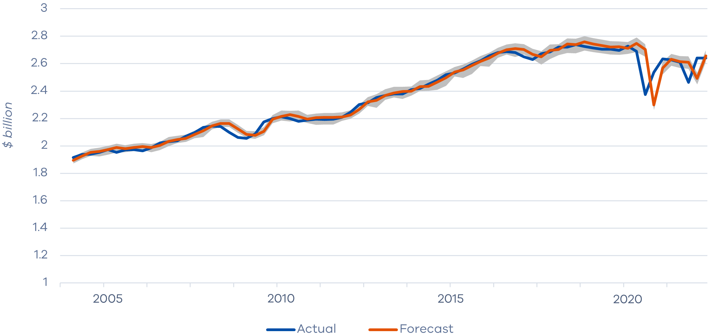
Figure 3: Consumption forecast versus actual
The shaded grey region represents the 95 per cent prediction interval for the single interval and refined AR‑MIDAS combination which consists of the following models: AR(2), MA(2), Optimised VAR, AR‑MIDAS underemployment and AR‑MIDAS credit card payment.
We consider our single interval benchmarks (AR2, MA2, VAR (optimised), VAR (literature)) plus our combinations of single‑interval and AR-MIDAS models (overall and refined). For illustrative purposes, Figure 3 plots forecasts and bootstrapped PIs for the single interval and refined AR‑MIDAS combination. Results show that actual values often lie within the PI. The point forecast is unable to identify the initial downturn at the beginning of both crises with consumption falling below the lower bound. Forecasts also lag behind the subsequent rebound with actual values violating the upper bound. Therefore, even though the MIDAS models and their combinations improve forecasts during crises, the challenge of accurately forecasting turning points remains.
To further assess our PIs, we examine whether PI violation rates are consistent with the 95 per cent confidence level. We perform the tests over the full OOS period and the OOS period excluding COVID‑19 and the GFC. We follow Kim et al. 2011 and test whether our PIs cover the actual out of sample values 95 per cent of the time. We calculate the mean coverage rate as:
where y is the actual value, L and U the lower and upper bounds of the PI, * denotes the frequency that the bracketed condition is satisfied, and T is the total number of prediction intervals. If the PI is accurate, C should be close to 0.95. To test whether C is statistically different to the nominal coverage of 0.95, we use a 95 per cent confidence interval based on a normal approximation to a binomial distribution:
where p=0.95. If C lies within this interval, we cannot reject the null that the actual coverage equals the nominal coverage at the 5 per cent level.
Over the entire OOS period, all models reject the null with coverage rates ranging from 74.7 per cent to 86.7 per cent. Our proposed PIs for the combinations of single-interval and MIDAS models have coverage rates similar to the conventional single interval models: 84.0 per cent (overall) and 81.3 per cent (refined). Given most PI violations occur over the crisis periods, we reconsider PI coverage rates over the OOS period excluding COVID‑19 and the GFC. All PIs now fail to reject the null.
In summary, results support the proposed bootstrap methodology when combining iterated and direct forecasts. PI violation rates for combinations of direct and iterated forecasts were consistent with the rates observed with conventional bootstrap methods for direct or iterated forecasts.
Table 3: 95 per cent prediction interval coverage rates
| Entire OOS period | Excluding OOS crisis periods | |
|---|---|---|
| Single interval models | ||
| AR(2) | 0.8533** | 0.9672 |
| MA(2) | 0.8667** | 0.9836 |
| Optimised VAR | 0.8667** | 0.9836 |
| Literature VAR | 0.7467** | 0.8689 |
| Single and mixed-interval model combinations | ||
| Overall | 0.8400** | 0.9508 |
| Refined | 0.8133** | 0.9180 |
Prediction interval coverage rate denotes the percentage of times the actual value is within the 95% confidence interval. ** indicates rejection of the null H0: the actual coverage rate = nominal coverage rate (0.95) at the 5% level of significance. The model combinations are equally weighted averages of the following models: 1) Overall: AR(2), MA(2), Optimised VAR, plus AR-MIDAS models fit to - credit card payments, consumer sentiment, underemployment, hours worked, house prices, cash rate target, credit card rate, savings rate, oil price and the trade-weighted-index; 2) Refined: AR(2), MA(2), Optimised VAR, AR-MIDAS underemployment and AR-MIDAS credit card payment.
High PI violation rates across all models and combinations was due to the inability of point forecasts to accurately predict turning points during crises. On removing crisis periods, the PI coverage rates were consistent with the level of confidence.
Finally, separate MIDAS models were constructed for each data category to assess their forecasts against the single-interval benchmarks. Table 3 reports DM tests that have been conducted across each data category with the best-performing MIDAS models. Direct measures of spending appear to be most valuable, with consistently positive t‑statistics. Financial market data is less informative despite its forward‑looking nature.
Table 4: MIDAS model Pairwise Diebold-Mariano tests
| Benchmarks | |||||||
|---|---|---|---|---|---|---|---|
| Credit Card | Sentiment | Underemp’t | House | Mortgage | Oil | Bal of trade | |
| Credit card | 1.28 | 1.05 | 1.54 | 1.60 | 0.81 | 1.49 | |
| Sentiment | -1.28 | -1.28 | 1.04 | 0.96 | -0.75 | -0.32 | |
| Underemp’t | -1.05 | 1.28 | 1.53 | 1.71* | 0.26 | 0.32 | |
| House | -1.54 | -1.04 | -1.53 | -0.50 | -1.04 | -0.67 | |
| Mortgage | -1.60 | -0.96 | -1.71 | 0.50 | -1.30 | -0.64 | |
| Oil | -0.81 | 0.75 | -0.26 | 1.04 | 1.30 | 0.19 | |
| Bal of trade | -1.49 | 0.32 | -0.32 | 0.67 | 0.64 | -0.19 | |
The t-statistic of the pairwise Diebold Mariano Tests conducted for each data category’s best MIDAS model against the benchmark denoted in each column is reported in the table above. A positive (negative) t-stat indicates that the model is better (worse) than the benchmark. * indicates the 10% significance level; ** indicates the 5% significance level and *** indicates the 1% significance level.
Footnotes
[1] The effect of consumer sentiment is proposed to occur through two main channels, the precautionary savings motive and the income growth expectations channel (Lahiri et al. 2016). There are consistent identification issues that prevent the first channel from being robustly identified. Souleles (2004) instead finds support for the effect of income growth expectations on consumer spending and observes significant heterogeneity in its effect across households. Fuhrer (1993) proposes the series lacks sufficient variation to be appropriately identified and Vosen and Schmidt (2011) suggest survey responses may not sufficiently capture the link between expectations and spending.
[2] Data supplied by Securities Industry Research Centre of Asia-Pacific (SIRCA) on behalf of CoreLogic.
[3] We use the AIC for lag determination. Most of the time, the lag was the same as that selected by the SIC, however in some instances we employed the SIC to save degrees of freedom.
[4] This is a modified version of the VAR model used by the Victorian Department of Treasury and Finance to forecast consumption.
[5] Models 3 and 4 (the VARs) are fitted at the quarterly frequency.
[6] Preference has been given to the RMSE as opposed to other loss functions like MAE, given the undesirability of large errors as consumption contributes such a large proportion of GDP.
[7] We also employed the model confidence set, which generally identified the same set of models.
[8] Future research could consider a model combination that dynamically weights forecasts from single‑interval and mixed‑interval models, depending on the current volatility of the economic environment as given by a market indicator such as the VIX.
Updated


